
5 minute read
Blurred lines: This is another entry in our irregular series on fundamental topics of light, colour and imaging. This time, we explore why there are so many different kinds of blur, why they differ in performance, and why one type that's found in almost every program is called Gaussian.
As the popularity of large-sensor cameras and short depth of field attests, blur can be beautiful. But the sort of blurs typically produced by real-world camera systems and those produced by computer software can be, and usually are, markedly different. In fact, one of the slowest blur filters in After Effects is called Camera Blur, and permits the user to define an iris shape and thereby simulate creative defocusing. The simulation is moderately coarse, failing to account for things like the common spherical distortion of the visible iris shape, although this can often be imitated using a combination of other filters.
Even so, almost all software offers a variety of blurs, from the quick-and-dirty box blur, through to advanced lens simulations.
To understand all this, we need to explore a few of the fundamentals of image processing. In the 1990s, it was quite common for software to offer the user raw and manual access to something called a convolution kernel, something that's available as Photoshop's “custom” filter. The most basic implementation of this comprises nine boxes, each of which may contain a digit, and an associated number called the divisor (or scale, or other terms).
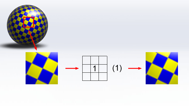
The reason that we don't use this construct very much anymore – at least in a way that's visible to the user – is that it's terribly counterintuitive, and there's no obvious clue as to how it works. The example kernel given above actually does nothing. To figure out what's going on, let's consider the convolution kernel that implements a three-pixel-square box blur:
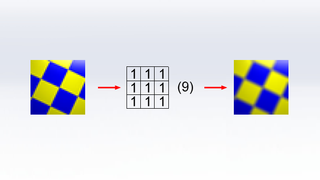
When the computer apples this kernel to an image, it considers each pixel in the input image in turn. The input pixel is represented by the central box. Each RGB value of the pixel is divided by the number on the right, then a proportion of the result of that division, controlled by the digit in each box, is added into the surrounding pixels. In this case, assuming the central pixel is full white, a value of one-ninth of full white will be written into each of the nine pixels involved in the kernel, producing a three-by-three blur. Larger kernels can produce larger blurs, such as this example which produces a five-by-five box blur:
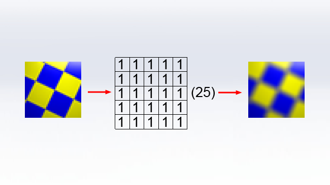
Again, each pixel in the input image is considered in terms of being the central pixel of the grid, and its value is divided by 25 then evenly distributed around the neighbouring pixels. Useful filters of other types, such as edge detection and embossing, can also be implemented as a convolution kernel, but we'll concentrate on blurring.
One of the problems with this simple approach to image processing is that it is very hard work. The value of each pixel must be retrieved from memory, divided, and then the values of nearby pixels retrieved and updated. For a five-by-five blur on a ten-megapixel image, then, two hundred and fifty million pixels must be handled (since 10 megapixels multiplied by 25 in each kernel is 250 million). Just retrieving and storing this many values is difficult, even overlooking the work of actually dividing and adding numbers together.
Modern CPUs have built-in fast memory that's intended to speed up jobs exactly such as this by keeping frequently-used values quickly to hand, but the average photographic image will be larger than the CPU's cache, leaving the computer to retrieve and store the data using the system's much slower main memory. Intelligent approaches can be designed to minimise the problem, but the situation remains less than ideal.
Worse, this is only a five-pixel blur. Larger blurs are possible but increasing size increases the workload proportionally to the square of the desired size (since 3x3=9, 5x5=25, etc). Performing a fifty-pixel blur on a ten-megapixel image using these techniques would require twenty-five billion pixel operations (since 50x50x10,000,000 = 25,000,000,000). And that's just for one RGB channel. Computers are good at crunching big sets of numbers, and the fact that all the kernel's values are one helps too, but this is becoming unreasonable.
The solution, as will be understood by people who've used the Motion Blur filter in Photoshop, is that the box blur can be separated into two much easier sequential operations. First, a blur in only the vertical axis, followed by a similar blur in the horizontal axis:
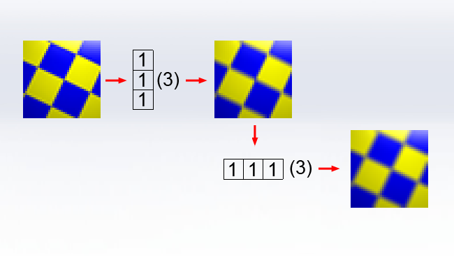
Even considering just a three-by-three blur, the workload is enormously reduced. As opposed to calculating and altering nine pixels for every input pixel, we modify only two sets of three, for a total of six. As the blur increases in size, the workload still increases, but it is proportional to the size doubled, as opposed to the size squared, which becomes a huge saving at larger sizes.
Unfortunately, this is still not an ideal solution. The results of a box blur invariably betray the inherent squareness of the kernel. In the theoretical circumstance of a single white input pixel against a black background, the output will be a perfect grey square. In some circumstances, particularly where there are small points of brightness in a photographic image, the boxiness of a box blur can become unacceptable. One solution to this is to fill the convolution kernel with a circular pattern of values, or at least as close to circular as is feasible. In both examples, the output has been brightened to make the effect more visible.
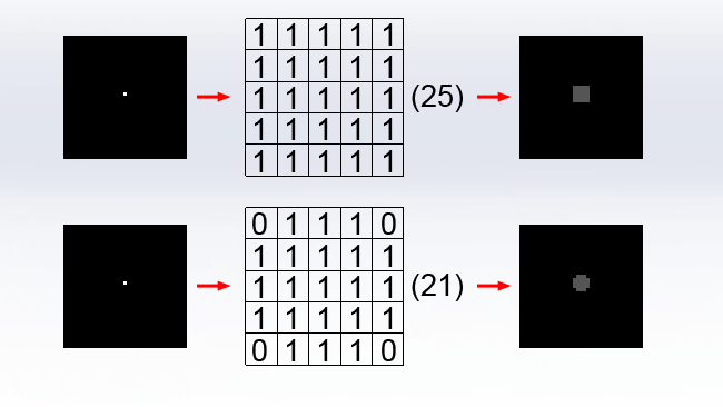
Of course, the “circle” created simply by setting the corner values of a five-by-five convolution kernel to zero is crude, but larger kernels naturally permit better resolution. It is also possible to implement antialiasing of the kernel by using values of less than 1, although that's overlooked here for simplicity. Notice that the divisor is reduced to 21 since there are now 21 values of one in the kernel – getting this wrong causes brightness shifts in the output.
The results from this type of blur – often rather imprecisely called a circular box blur – can quite closely approximate real camera blur, but there's a problem: we can no longer separate the blur into a horizontal and vertical pass, because not all the rows and columns are now the same, and we have no choice but to do all of the calculations with sheer number crunching brute force.
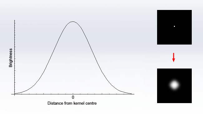
The Gaussian function is a piece of mathematics developed by Carl Friedrich Gauss, one of the most important and influential figures in mathematics, and pops up in all sorts of real-world situations. The graph of the function is the familiar bell curve, which is so commonly encountered in real-world statistics that it's referred to in the field as the normal distribution:
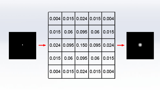
The reason it's important in image processing, however, is that the Gaussian is a function that is separable and can be broken down into two one-dimensional operations, yet produces a circular blur. If we sample the Gaussian function in two dimensions to create a convolution kernel, we get this (Again, the output has been brightened for clarity, and the values are given fractionally so the divisor is always 1):
But we can achieve identical results by doing a much simpler operation, twice, horizontally and vertically:
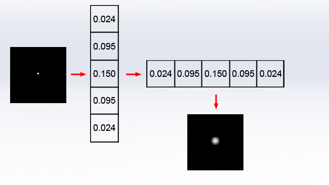
There are other solutions. A box blur, which is still faster to calculate than Gaussian because its kernel consists of only one repeated value, can be applied repeatedly to an image. Applying a box blur three times very approximates a Gaussian blur to within a few percent (the proof is in the Central Limit Theorem, which states that this sort of thing tends towards a normal distribution, which as the statisticians know is Gaussian).
But in the end, that's why computers use Gaussian blurs a lot. It's not because they particularly simulate any real-world optical effect – they don't – it's because they are reasonably fast to render and not too ugly.
Tags: Technology

RedShark 2020 @ All rights reserved.

Comments